
In earlier blog posts we described what time series data is and key characteristics of a time series database. In this blog post, which originally appeared in The New Stack, Eric Hanson, principal product manager at SingleStore, shows you how to use SingleStore for time series applications.
At SingleStore we’ve seen strong interest in using our database for time series data. This is especially the case when an organization needs to accommodate the following: (1) a high rate of event ingestion, (2) low-latency queries, and (3) a high rate of concurrent queries.
In what follows, I show how SingleStore can be used as a powerful time-series database and illustrate this with simple queries and user-defined functions (UDFs) that show how to do time series-frequency conversion, smoothing, and more. I also cover how to load time series-data points fast, with no scale limits.
Note: This blog post was originally published in March 2019. It has been updated to reflect the new time series functions in SingleStoreDB Self-Managed 7.0. Please see the Addendum at the end of this article for specifics on using the information herein. – Ed.
Manipulating Time Series with SQL
Unlike most time series-specific databases, SingleStore supports standard SQL, including inner and outer joins, subqueries, common table expressions (CTEs), views, rich scalar functions for date and time manipulation, grouping, aggregation, and window functions. We support all the common SQL data types, including a datetime(6) type with microsecond accuracy that’s perfect as a time series timestamp.
A common type of time-series analysis in financial trading systems is to manipulate stock ticks. Here’s a simple example of using standard SQL to do this kind of calculation. We use a table with a time series of ticks for multiple stocks, and produce high, low, open, and close for each stock:
CREATE TABLE tick(ts datetime(6), symbol varchar(5),
   price numeric(18,4));
INSERT INTO tick VALUES
  ('2019-02-18 10:55:36.179760', 'ABC', 100.00),
  ('2019-02-18 10:57:26.179761', 'ABC', 101.00),
  ('2019-02-18 10:59:16.178763', 'ABC', 102.50),
  ('2019-02-18 11:00:56.179769', 'ABC', 102.00),
  ('2019-02-18 11:01:37.179769', 'ABC', 103.00),
  ('2019-02-18 11:02:46.179769', 'ABC', 103.00),
  ('2019-02-18 11:02:59.179769', 'ABC', 102.60),
  ('2019-02-18 11:02:46.179769', 'XYZ', 103.00),
  ('2019-02-18 11:02:59.179769', 'XYZ', 102.60),
  ('2019-02-18 11:03:59.179769', 'XYZ', 102.50);
This query uses standard SQL window functions to produce high, low, open and close values for each symbol in the table, assuming that “ticks” contains data for the most recent trading day.
WITH ranked AS
(SELECT symbol,
    RANK() OVER w as r,
    MIN(price) OVER w as min_pr,
    MAX(price) OVER w as max_pr,
    FIRST_VALUE(price) OVER w as first,
    LAST_VALUE(price) OVER w as last
    FROM tick
    WINDOW w AS (PARTITION BY symbol
    ORDER BY ts
        ROWS BETWEEN UNBOUNDED PRECEDING
        AND UNBOUNDED FOLLOWING))

SELECT symbol, min_pr, max_pr, first, last
FROM ranked
WHERE r = 1;
Results:
+--------+----------+----------+----------+----------+
| symbol | min_pr   | max_pr   | first    | last     |
+--------+----------+----------+----------+----------+
| XYZ    | 102.5000 | 103.0000 | 103.0000 | 102.5000 |
| ABC    | 100.0000 | 103.0000 | 100.0000 | 102.6000 |
+--------+----------+----------+----------+----------+
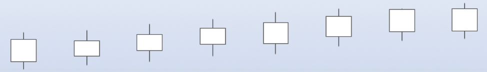
Similar queries can be used to create “candlestick charts,” a popular report style for financial time series that looks like the image below. A candlestick chart shows open, high, low, and close prices for a security over successive time intervals:
For example, this query generates a table that can be directly converted to a candlestick chart over three-minute intervals:
WITH ranked AS
   (SELECT symbol, ts,
    RANK() OVER w as r,
    MIN(price) OVER w as min_pr,
    MAX(price) OVER w as max_pr,
    FIRST_VALUE(price) OVER w as first,
    LAST_VALUE(price) OVER w as last

   FROM tick
   WINDOW w AS (PARTITION BY symbol, time_bucket('3 minute', ts)
        ORDER BY ts
        ROWS BETWEEN UNBOUNDED PRECEDING
                AND UNBOUNDED FOLLOWING))

SELECT symbol, time_bucket('3 minute', ts), min_pr, max_pr,
first, last
FROM ranked
WHERE r = 1
ORDER BY 1, 2;
Results:
+--------+-----------------------------+----------+----------+----------+----------+
| symbol | time_bucket('3 minute', ts) | min_pr   | max_pr   | first    | last     |
+--------+-----------------------------+----------+----------+----------+----------+
| ABC    | 2019-02-18 10:54:00.000000  | 100.0000 | 100.0000 | 100.0000 | 100.0000 |
| ABC    | 2019-02-18 10:57:00.000000  | 101.0000 | 102.5000 | 101.0000 | 102.5000 |
| ABC    | 2019-02-18 11:00:00.000000  | 102.0000 | 103.0000 | 102.0000 | 102.6000 |
| XYZ    | 2019-02-18 11:00:00.000000  | 102.6000 | 103.0000 | 103.0000 | 102.6000 |
| XYZ    | 2019-02-18 11:03:00.000000  | 102.5000 | 102.5000 | 102.5000 | 102.5000 |
+--------+-----------------------------+----------+----------+----------+----------+
Smoothing is another common need in managing time series data. This query produces a smoothed sequence of prices for stock “ABC,” averaging the price over the last three ticks:
SELECT symbol, ts, price,
AVG(price) OVER (ORDER BY ts ROWS BETWEEN 3 PRECEDING AND CURRENT ROW) AS smoothed_price
FROM tick
WHERE symbol = 'ABC';
Results:
+--------+----------------------------+----------+----------------+
| symbol | ts                         | price    | smoothed_price |
+--------+----------------------------+----------+----------------+
| ABC    | 2019-02-18 10:55:36.179760 | 100.0000 |   100.00000000 |
| ABC    | 2019-02-18 10:57:26.179761 | 101.0000 |   100.50000000 |
| ABC    | 2019-02-18 10:59:16.178763 | 102.5000 |   101.16666667 |
| ABC    | 2019-02-18 11:00:56.179769 | 102.0000 |   101.37500000 |
| ABC    | 2019-02-18 11:01:37.179769 | 103.0000 |   102.12500000 |
| ABC    | 2019-02-18 11:02:46.179769 | 103.0000 |   102.62500000 |
| ABC    | 2019-02-18 11:02:59.179769 | 102.6000 |   102.65000000 |
+--------+----------------------------+----------+----------------+
Using Extensibility to Increase the Power of SingleStore for Time Series
SingleStore supports extensibility with user-defined functions and stored procedures. SingleStore compiles UDFs and stored procedures to machine code for high performance.
I actually used SingleStore’s extensibility to create the time_bucket() function, shown in the Supplemental Material section below, which appeared in the previous section as a UDF. This function provides equivalent capability to similar functions in time-series-specific products. You can easily create a function or expression to bucket by time intervals, such as second, minute, hour, or day.
A common need with time-series data is to perform interpolation. For example, suppose you have a time series with points at random intervals that are 30 seconds apart on average. There may be some minutes with no data point. So, if you convert the raw (irregular) time-series data to a regular time series with a point a minute, there may be gaps.
If you want to provide output for plotting with no gaps, you need to interpolate the values for the gaps from the values before and after the gaps. It’s straightforward to implement a stored procedure in SingleStore by taking a query result and outputting a row set, with the gaps interpolated, into a temporary table.
This can then be sent back to the client application using the ECHO command. In addition, SingleStore supports user-defined aggregate functions. These functions can be used to implement useful time series operations, such as shorthand for getting the first and last values in a sequence without the need for specific window functions.
Consider this query to get the first value for stock ABC in each three minutes of trading, based on a user-defined aggregate function (UDAF) called FIRST():
SELECT time_bucket('3 minute', ts), first(price, ts)
FROM tick
WHERE symbol = "ABC"
GROUP BY 1
ORDER BY 1;
Results:
+-----------------------------+------------------+
| time_bucket('3 minute', ts) | first(price, ts) |
+-----------------------------+------------------+
| 2019-02-18 10:54:00.000000  | 100.0000         |
| 2019-02-18 10:57:00.000000  | 101.0000         |
| 2019-02-18 11:00:00.000000  | 102.0000         |
+-----------------------------+------------------+
The implementations of the FIRST() UDAF, and the analogous LAST() UDAF, are shown in the Supplemental Material section below.
Time Series Compression and Life Cycle Management
SingleStore is adept at handling both bursty insert traffic for time series events and historical time series information where space savings are important. For bursty insert traffic, you can use a SingleStore rowstore table to hold time series events.
For larger and longer-lived sets of time series events, or older time series data sets that have aged and are unlikely to be updated anymore, the SingleStore columnstore is a great format. It compresses time-series data very effectively, with SingleStore supporting fast operations on compressed columnstore data. Moreover, columnstore data resides on disk, so main memory size is not a limit on how much data you can store.
Scalable Time Series Ingestion
When building a time series application, data can come at high rates from many sources. Sources include applications, file systems, AWS S3, Hadoop HDFS, Azure Blob stores, and Kafka queues. SingleStore can ingest data incredibly fast from all these sources.
SingleStore Pipelines are purpose-built for fast and easy loading of data streams from these sources, requiring no procedural coding to establish a fast flow of events into SingleStore.
SingleStore can ingest data at phenomenal data rates. In a recent test, I inserted 2,850,500 events per second directly from an application, with full transactional integrity and persistence, using a two-leaf SingleStore cluster. Each leaf ran on an Intel Xeon Platinum 28-core system.
Comparable or even better rates can be had using direct loading or Kafka pipelines. If you have to scale higher, just add more nodes — there’s no practical limit.
When General-Purpose SingleStore Is Right for Time Series
We’ve seen the market for time-series data management bifurcate into special-purpose products for time series, with their own special-purpose languages, and extended SQL systems that can interoperate with standard reporting and business intelligence tools that use SQL. SingleStore is in this second category.
SingleStore is right for time series applications that need rapid ingest, low-latency query, and high concurrency, without scale limits, and which benefit from SQL language features and SQL tool connectivity.
Many time-series-specific products have shortcomings when it comes to data management. Some lack scale-out, capping the size of problems they can tackle, or forcing application developers to build tortuous sharding logic into their code to split data across multiple instances, which costs precious dollars for labor that could better be invested into application business logic.
Other systems have interpreted query processors that can’t keep up with the latest query execution implementations as ours can. Some lack transaction processing integrity features common to SQL databases.
SingleStore lets time series application developers move forward confidently, knowing they won’t hit a scale wall, and they can use all their familiar tools — anything that can connect to a SQL database.
Summary
SingleStore is a strong platform for managing time series data. It supports the ability to load streams of events fast and conveniently, with unlimited scale. It supports full SQL that enables sophisticated querying using all the standard capabilities of SQL 92, plus the more recently added window function extensions.
SingleStore supports transactions, high rates of concurrent update and query, and high availability technologies that many developers need for all kinds of applications, including time series. And your favorite SQL-compatible tools, such as business intelligence (BI) tools, can connect to SingleStore. Users and developers – in areas such as real-time analytics, predictive analytics, machine learning, and AI – can use the SQL interfaces they’re familiar with, as described above. All of this and more makes SingleStore a strong platform for time series.
Download and use SingleStore for free today and try it on your time series data!
Addendum
In SingleStoreDB Self-Managed 7.0, we added TIME_BUCKET(), FIRST(), and LAST() as built-in functions. So, if you run the scripts above to create those functions on SingleStoreDB Self-Managed 7.0, you will get an error. We recommend that you simply use the built-in version of the functions in 7.0. See the documentation here: https://archived.docs.singlestore.com/v7.0/reference/sql-reference/time-series-functions/time-series-functions/
If you’d like to experiment with the user-defined versions, edit the scripts to rename the functions to TIME_BUCKET2(), FIRST2(), and LAST2(), or something similar, before creating them.
Supplemental Material 1/2: Full Text of time_bucket() Function
-- Usage: time_bucket(interval_string, timestamp_value)
-- Examples: time_bucket('1 day', ts), time_bucket('5 seconds', ts)

DELIMITER //
CREATE OR REPLACE FUNCTION time_bucket(
  bucket_desc varchar(64) NOT NULL,
  ts datetime(6)) RETURNS datetime(6) NULL AS
DECLARE
  num_periods bigint = -1;
  second_part_offset int = -1;
  unit varchar(255) = NULL;
  num_str varchar(255) = NULL;
  unix_ts bigint;
  r datetime(6);
  days_since_epoch bigint;
BEGIN
  num_str = substring_index(bucket_desc, ' ', 1);
  num_periods = num_str :> bigint;
  unit = substr(bucket_desc, length(num_str) + 2, length(bucket_desc));
  IF unit = 'second' or unit = 'seconds' THEN
    unit = 'second';
  ELSIF unit = 'minute' or unit = 'minutes' THEN
    unit = 'minute';
  ELSIF unit = 'hour' or unit = 'hours' THEN
    unit = 'hour';
  ELSIF unit = 'day' or unit = 'days' THEN
    unit = 'day';
  ELSE
    raise user_exception(concat("Unknown time unit: ", unit));
  END IF;

  unix_ts = unix_timestamp(ts);

  IF unit = 'second' THEN
    r = from_unixtime(unix_ts - (unix_ts % num_periods));
  ELSIF unit = 'minute' THEN
    r = from_unixtime(unix_ts - (unix_ts % (num_periods * 60)));
  ELSIF unit = 'hour' THEN
    r = from_unixtime(unix_ts - (unix_ts % (num_periods * 60 * 60)));
  ELSIF unit = 'day' THEN
    unix_ts += 4 * 60 * 60; -- adjust to align day boundary
    days_since_epoch = unix_ts / (24 * 60 * 60);
    days_since_epoch = days_since_epoch - (days_since_epoch % num_periods);
    r = (from_unixtime(days_since_epoch * (24 * 60 * 60))) :> date;
  ELSE
    raise user_exception("Internal error -- bad time unit");
  END IF;

  RETURN r;
END;
//
DELIMITER ;
Supplemental Material 2/2: Full Text of first() and last() Aggregate Functions
The following UDAF returns the first value in a sequence, ordered by the second argument, a timestamp:
-- Usage: first(value, timestamp_expr)
-- Example:
--   Get first value of x for each day from a time series in table
--     t(x, ts)
--   with timestamp ts.
--
--   SELECT ts :> date, first(x, ts) FROM t GROUP BY 1 ORDER BY 1;

DELIMITER //
CREATE OR REPLACE FUNCTION first_init() RETURNS RECORD(v TEXT, d datetime(6)) AS
  BEGIN
    RETURN ROW("_empty_set_", '9999-12-31 23:59:59.999999');
  END //
DELIMITER ;

DELIMITER //
CREATE OR REPLACE FUNCTION first_iter(state RECORD(v TEXT, d DATETIME(6)),
   v TEXT, d DATETIME(6))
  RETURNS RECORD(v TEXT, d DATETIME(6)) AS
  DECLARE
    nv TEXT;
    nd DATETIME(6);
    nr RECORD(v TEXT, d DATETIME(6));
  BEGIN
    -- if new timestamp is less than lowest before, update state
    IF state.d > d THEN
      nr.v = v;
      nr.d = d;
      RETURN nr;
    END IF;
    RETURN state;
  END //
DELIMITER ;

DELIMITER //
CREATE OR REPLACE FUNCTION first_merge(state1 RECORD(v TEXT, d DATETIME(6)),
   state2 RECORD(v TEXT, d DATETIME(6))) RETURNS RECORD(v TEXT, d DATETIME(6)) AS
  BEGIN
    IF state1.d < state2.d THEN
      RETURN state1;
    END IF;
    RETURN state2;
  END //
DELIMITER ;

DELIMITER //
CREATE OR REPLACE FUNCTION first_terminate(state RECORD(v TEXT, d DATETIME(6))) RETURNS TEXT AS
  BEGIN
    RETURN state.v;
  END //
DELIMITER ;

CREATE AGGREGATE first(TEXT, DATETIME(6)) RETURNS TEXT
  WITH STATE RECORD(v TEXT, d DATETIME(6))
  INITIALIZE WITH first_init
  ITERATE WITH first_iter
  MERGE WITH first_merge
  TERMINATE WITH first_terminate;
A LAST() UDAF that is analogous to FIRST(), but returns the final value in a sequence ordered by timestamp, is as follows:
-- Usage: last(value, timestamp_expr)
-- Example:
--   Get last value of x for each day from a time series in table t
--     t(x, ts)
--   with timestamp column ts.
--
--   SELECT ts :> date, last(x, ts) FROM t GROUP BY 1 ORDER BY 1;

DELIMITER //
CREATE OR REPLACE FUNCTION last_init() RETURNS RECORD(v TEXT, d datetime(6)) AS
  BEGIN
    RETURN ROW("_empty_set_", '1000-01-01 00:00:00.000000');
  END //
DELIMITER ;

DELIMITER //
CREATE OR REPLACE FUNCTION last_iter(state RECORD(v TEXT, d DATETIME(6)),
   v TEXT, d DATETIME(6))
  RETURNS RECORD(v TEXT, d DATETIME(6)) AS
  DECLARE
    nv TEXT;
    nd DATETIME(6);
    nr RECORD(v TEXT, d DATETIME(6));
  BEGIN
    -- if new timestamp is greater than largest before, update state
    IF state.d < d THEN nr.v = v; nr.d = d; RETURN nr; END IF; RETURN state; END // DELIMITER ; DELIMITER // CREATE OR REPLACE FUNCTION last_merge(state1 RECORD(v TEXT, d DATETIME(6)), state2 RECORD(v TEXT, d DATETIME(6))) RETURNS RECORD(v TEXT, d DATETIME(6)) AS BEGIN IF state1.d > state2.d THEN
      RETURN state1;
    END IF;
    RETURN state2;
  END //
DELIMITER ;

DELIMITER //
CREATE OR REPLACE FUNCTION last_terminate(state RECORD(v TEXT, d DATETIME(6))) RETURNS TEXT AS
  BEGIN
    RETURN state.v;
  END //
DELIMITER ;

CREATE AGGREGATE last(TEXT, DATETIME(6)) RETURNS TEXT
  WITH STATE RECORD(v TEXT, d DATETIME(6))
  INITIALIZE WITH last_init
  ITERATE WITH last_iter
  MERGE WITH last_merge
  TERMINATE WITH last_terminate;